Introduction
Note: “.” is used for the decimal point and “,” is the thousands separator.
This second installment on data plumbing will tackle the interplay between protein inference and quantitative data rollup in shotgun proteomics. The discussion will be about the general problem of how we try to put Humpty Dumpty back together again; i.e. how do we form protein expression values from measurements of peptide spectrum matches (PSMs) or MS1 features.
We frequently do these discovery shotgun quantification experiments when we are characterizing systems where there is not much prior knowledge. We want to get some insight into biological process and pathway differences in response to system perturbations. Most biological effects occur via multi-protein mechanisms (pathways, complexes, and interactions). We tend to focus less on single, specific proteins so that we can get global views of the system.
These global approaches make many simplifying assumptions, and can, therefore, have some limitations. We need to review the basic steps in shotgun quantification first in order to understand when limitations might arise. We will talk some about limitations at the end.
Shotgun quantification methods are all similar
Many people might think spectral counting, intensity-weighted spectral counting (also this reference), accurate mass and time (AMT) tag methods, MaxQuant LFQ, MaxQuant iBAQ, SILAC, iTRAQ, and TMT are all rather different quantitative proteomics techniques. If you take a step back, no - a bigger step, keep going, STOP!, you might see that all shotgun quantitation methods are just weighted spectral counting with different weights. First, I need to climb onto my soapbox and
Rant against ratios: We are going to be spending a lot of time talking about rolling up lower level measurements to higher levels (like proteins). We are not going to talk about ratios, median ratios, signal-to-noise ratios, golden ratios, the 80:20 ratio, pi, or any other kind of ratios. Ratios and statistics do not mix (ask any statistician). We want quantitative proteomics to be serious quantitative work; something that uses real statistics so that we can say this result is significant.
Ratio drawbacks: There are few reasons to use ratios and many reasons not to use them. Measurements are made on some natural scale that has physical meaning. We often have good intuition about the data in its natural scale. Ratios change the natural scale. Ratios compress the range of the numbers. Half of the ratios are between 0 and one. The other half are between 1 and infinity. This asymmetry in numerical values is “fixed” by taking the logarithms of the values. This further compresses the range of values. No one on this planet has any intuition about numbers in reciprocal or logarithmic spaces. There are no reasons to work with ratios (in most cases) other than this being the poor way that quantitative proteomics has been done in the past.
What all of these methods have in common is that we have proteins in our samples, but we do not make measurements of proteins. We choose to digest the proteins and measure the liberated peptides instead. What are the relationships of the measured peptides to the proteins originally in the sample? The answer is not 42; it depends on a lot of things.
Context is everything
A (tryptic) peptide is pretty short, so the amino acid sequence may not be unique. Unique is defined in this context as the peptide mapping to a single gene product (a protein). It is not a simple case of peptide length for uniqueness; although longer peptides are more likely to be unique. Nature, unlike humans, tries to recycle things. There are motifs in proteins that do useful things and these tend to be conserved. We can have conserved motifs between different proteins within the same organism and we can have conserved motifs between species.
It is becoming more rare to have data from a species that does not have a sequenced genome. It is also possible now to create custom genomes for the samples being studied. One context is the genome of the samples under study, another is the available sequenced genome from one of the genomic sequence warehouses. There are additional contexts that come from predicting the protein sequences coded by the genomic sequences. The protein FASTA file used in analyzing your data is not the only genomic context for your samples.
Higher eukaryotic organisms have genes that produce multiple, similar protein products to increase functional diversity. These protein isoform families can liberate many peptides that are the same after digestion. There can be more complete (isoforms present) or canonical (single gene products) FASTA databases to choose from. Most organisms also try to cheat death by having multiple protein coding genes for critical housekeeping functions. The duplicated genes can produce identical or nearly identical gene products. Many peptide sequences identified in shotgun studies can come from more than one protein.
What is the relationship of these shared peptides to the proteins, and what can we say about the measured values for these shared peptides? The bottom line is that the information content is different for unique and shared peptides. In next generation mRNA sequencing, they just toss out the shared reads. We can have a lot of shared peptides in proteomics, so we generally avoid tossing them out.
Shotgun quantification boils down to how do we define shared and unique peptides, in what context, and what do we do with the shared peptides. This creates a tension between quantitative resolution (how finely can we quantify proteins or even parts of proteins) and trying to recover as much quantitative information from the shared peptides as possible. We worry about the later situation because many proteins in shotgun experiments are not abundant and we have limited measurements for them. Discarding shared peptides too aggressively can compromise the data quality. How we make decisions about the shared peptides depends on the protein inference process.
This is how shotgun quantification and protein inference are intimately coupled. You might have a biological question where maintaining lots of quantitative resolution is much more important than trying to reduce noise and simplify the results. Lucky you! You can stop reading this. However, most pipelines such as mine, or Proteome Discoverer, or MaxQuant, or Scaffold are going to make efforts to recover quantitative information from shared peptides. Keep reading if you want to gain some understanding of how that is done.
Relevant pipeline steps
I did a blog post about pipelines where typical processing steps were outlined. Most upstream steps are about filtering PSMs with some acceptable error rate, typically 1%. If you had 250,000 MS2 scans and could identify 40% of those (these are pretty typical numbers for shotgun experiments on Orbitraps), you would have 100,000 PSMs after filtering out most of the incorrect matches. A 1% FDR implies that there would be 1,000 incorrect PSMs. You do not know which of the 100,000 PSMs might be the 1,000 incorrect ones. Would you trust the quantitative information from those 1,000 PSMs?
Protein inference
Generally, we combine proteins having (mass spec) indistinguishable sets of matching peptides into single groups, and remove any proteins whose set of peptides can be explained by other proteins (with larger peptide sets). This constitutes basic parsimony principles. We (usually) do not have more than one identical protein sequence in the FASTA protein database file. While the protein sequences tend to always be unique, because we only observe partial sequence coverage, the observed peptides may not be capable of distinguishing proteins. Our ability to distinguish proteins is reduced as sequence coverage decreases. We know that PSM counts are correlated with abundance, so we have better odds of distinguishing abundant proteins (where coverage is higher) compared to lower abundance proteins.
Each biological sample starts with intact proteins that get digested into peptides. Strictly speaking, we should map peptides to proteins separately for each biological sample. We do not know for sure if peptides coming from different biological samples came from the same protein because we do not know what proteins are present in each different sample yet. Unfortunately, many proteins have few peptides and whether or not those peptides are distinguishable can vary sample-to-sample. This can make aligning identifications between samples challenging.
A strategy that kills two birds with one stone is to collectively map all of the peptides from all of the samples in an experiment-wide protein inference process. This gives more sequence coverage to make identical set and subset calls. It also takes care of aligning protein identifications across all samples in the experiment. We may need to do some per sample cleanup if we have some minimum protein identification criteria to meet. This strategy tends to minimize protein grouping in basic parsimony logic. It can lead to proteins that are indistinguishable in a given sample being reported as distinguishable despite each protein has no unique peptides (this seems rare in my experience). Every choice has its consequences.
Protein error control
As we have moved through the data processing steps, we have reduced the number of PSMs by rejecting the majority of the incorrect matches. We have mapped those peptide sequences to the protein sequences that were in the FASTA file and followed some parsimony rules to simplify the protein list. Remember that we still have incorrect PSMs that might lead to incorrect protein identifications to deal with.
There are two ways to control the number of incorrect proteins: ad hoc ranking functions or basic probability theory. Ad hoc ranking functions approach the problem like it is similar to the statistical treatment of PSM scores. It is not. While a target or decoy protein counting does give some ballpark estimate of the protein error rate, there are insufficient numbers of target and (especially) decoy proteins for any valid statistical assessment. You would need to know the decoy protein score distribution and that is not possible because nearly all incorrect PSMs have been filtered out.
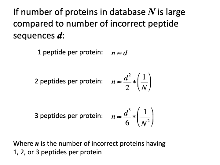
The process by which incorrect peptide sequences manifest as incorrect protein sequences is not at all like how incorrect PSM scores end up in the correct pile. We all know that the number of peptides per protein is somehow important. That is how the two-peptide rule came to pass. The Supplemental materials for the MAYU paper worked out the basic probability equation.
The formula can be simplified for the typical proteomics case. If we just want to get the gist of how numbers of incorrect proteins depend on numbers of incorrect peptides, we can make some approximations. The number of incorrect peptide sequences are usually much smaller than the number of proteins in the FASTA database. The numbers of incorrect peptides are typically a few hundred to a thousand. The number of proteins in protein databases are typically many tens of thousands. Consequently, one of the terms in the hypergeometric probability equation will be so close to 1.0 that we can drop it. Truncated factorials can be replaced with power expressions (100 x 99 x 98 is pretty close to 100^3). There is explicit dependence on the number of peptides per protein. The number of incorrect proteins drops off so rapidly with increasing numbers of peptides per protein, that explicit forms for 1, 2 or 3 peptides per protein are all that are relevant.
There are a few key points:
- there is a direct dependence on number of incorrect peptides
- there is an inverse relationship with the protein database size
- formulae predict the number of incorrect proteins
- single peptide per protein IDs have a one-to-one error relationship
- three peptides per protein error numbers are typically very small
- two peptides per protein is the sweet spot
There are some caveats
- lengths of the protein sequences are ignored
- database size should be proportional to theoretical peptide search space
- incorrect matches to correct proteins are ignored
These formulae are in the ballpark if the number of proteins identified in the sample are a reasonably small fraction of the database size. Scalings of the estimates have to be done if the numbers of protein IDs become too large compared to the target database.
With the typical numbers mentioned above, the 1,000 incorrect PSMs would result in 1,000 incorrect proteins if we allowed single peptide per protein IDs (without ranking functions and an FDR analysis). We would only have a handful of incorrect proteins (estimate of 25 for a 20,000 sequence protein database) with the two-peptide rule. Protein ranking functions are untested and could suffer from inaccurate error estimates given the fluctuations in counts of small numbers. The two-peptide rule is derived from simple probability theory and effectively controls the number of incorrect proteins.
Shared peptides are a moving target
The proteins that the measured peptides suggest could be present in our sample are not a simple subset of the starting FASTA file. We have peptide ambiguity and we have partial sequence coverage. We have groups of indistinguishable proteins, individual distinguishable proteins, and rejected proteins that we thought we did not have enough evidence to report. We also have some peptide errors.
See the 2005 definitive paper on protein inference for definitions of the terminology.
We started by mapping peptide sequences to the protein sequences in the FASTA file. Peptides that mapped to a single protein sequence were unique, and those that mapped to more than one were shared. We formed peptide sets for each of the proteins pointed to by any of the identified peptides. We compared peptide sets to determine distinguishable proteins, indistinguishable protein groups, and remove proteins with subset peptide sets. That defines a new context for defining shared and unique peptides with respect to the parsimonious list of proteins inferred in the experiment. Many of the peptides in indistinguishable protein groups, which were all shared in the context of the FASTA file, become unique peptides in the new context.
These days most datasets are enormous. We identify a large number of PSMs at fixed false discovery rates. That can lead to not insignificant numbers of incorrect peptides. These large numbers of identified peptides result in large number of proteins being inferred (reports of 5,000 to 10,000 proteins in studies are not uncommon). It becomes more likely that correct proteins can have incorrect associated peptides. Those stray matches can throw a wrench into the parsimony logic. We might have identical peptides sets no longer being identical or not remove a subset because of an incorrect peptide match. We need to add a little fuzziness to the parsimony logic.
We can define extended parsimony logic to allow grouping of proteins having nearly identical peptide sets. We can remove proteins if their peptide set are nearly fully contained in larger peptide sets. We can circle back to the two-peptide rule to help us define nearly. If we have less than one or two unique peptides and a lot of shared peptides, we can group those proteins (or remove as a subset). We can still have abundant, highly homologous housekeeping proteins where we may have mostly shared peptides and just a few unique peptides. When the shared peptides dominate, it might be safer to lump the proteins into a single family, and quantify the family rather than the family members.
Once again, we redefine shared and unique peptides after doing the extended parsimony analysis. This also changes many formerly shared peptides to unique peptides and increases the quantitative information content of the experiment that we can use.
There are alternative ways to group similar proteins that are implemented in Scaffold and Mascot. These may seem like some really bad ideas given what we know about some proteins in some biological systems. The truth is that the alternatives are worse. Without grouping, we have predominantly shared peptides that we cannot use for quantification. The leftover unique peptides may be low abundance or even incorrect matches. The quantification would be unreliable in many cases.
The razor peptide concept implemented in Proteome Discover, MaxQuant, and other pipelines is kind of a one good protein and all of the others end up bad situation. It is like one protein of a family gets a gigantic job promotion to the razor protein. It gets all of the shared peptides. The other family members get little or nothing. They are left with the shirt on their backs (their unique peptides) to fend for themselves. One protein ends up with a really nice house on easy street and the others are left scrounging dumpsters. It can be difficult in results files to figure out which are the poor proteins with poor quantitative information.
Where are we at and where are we going?
The discussion so far has not had included much of anything about quantitative data. It has all been about how we define the relationships between peptides and proteins in shotgun experiments. The process of going from MS2 spectra to PSMs to peptides to proteins creates a variety of contexts that affect how we defined shared and unique peptide status. At the end of all of this, we finally know enough about the information content of each peptide that we can decide what to do with their associated quantitative data.
You can think of the protein inference and definitions of unique peptides in the proper context as creating a scaffolding that we can add the quantitative measurements to. There are differentially expressed features in datasets that are not identified. As techniques have improved and larger fractions of data have assigned PSMs, we have moved from “quantify first and identify later” thinking to “just quantify what we identify”. We have become quite dependent on protein inference informing and guiding shotgun quantitative experiments.
We are now faced with many choices about how to proceed with the quantitative data. A motivation for this blog was to shed some light on how discovery quantification differs from more targeted quantification strategies. In discovery phase, we are trying to learn more about our system so we can form more directed hypotheses. Only when we have some concrete hypotheses can we formulate more precise questions to guide targeted studies. There may be many situations where the strategies discussed below will be wrong and lead to incorrect conclusions. A very interesting question is whether or not there is some signature in discovery data that can suggest when its assumptions are being violated. The first thing is to try and describe how to aggregate PSM-level quantitative data into protein-level summaries. We have to understand that before we can dissect the fundamental differences between discovery and target quantification strategies.
This is where we come to forks in the road. There are many choices for how to relate measurements of the abundances of pieces of the protein to estimates of the whole protein abundance. One way to categorize the choices is by what kind of abundance they seem to be measuring. Common abundance scales used in proteomics are molar concentrations and percentage scales (weight or volume). Things like the top 3 method, NSAF spectral counting, or iBAQ are more like molar concentrations. Spectral counting, MaxQuant LFQ, TMT in MaxQuant or Proteome Discoverer or my pipeline are more like weight percentages.
We often need large scale peptide separations in discovery phase because we do not know ahead of time if the interesting players will be high, medium, or low abundance proteins. Methods that require more specific measurements of an analyte’s signal need to have more reproducible chromatography conditions that can be at odds with large-scale separations. Weight percentage methods are essentially “lump everything we measure about a protein together”, so they are more forgiving of large-scale separations.
How to “lump everything together”
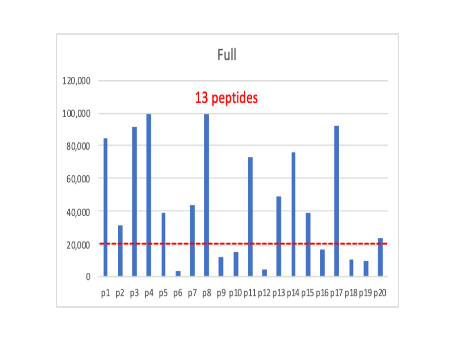
In spectral counting, the numbers of PSMs associated with a protein are proportional to the protein’s abundance. In a great oversimplification, this is because instruments have a linear measurement range and a lower limit of detection. If a protein is more abundant, all of its pieces will tend to be more abundant. More of the pieces will have signals that fall above the detection limit. As the overall protein abundance decreases, more of the pieces fall below the limit leaving fewer above the limit. The figures below are for a hypothetical protein having 20 peptides. The signals are random values between zero and 100,000 for the Full plot. The red dotted line represents the detection limit. We have 13 peptides above the limit.
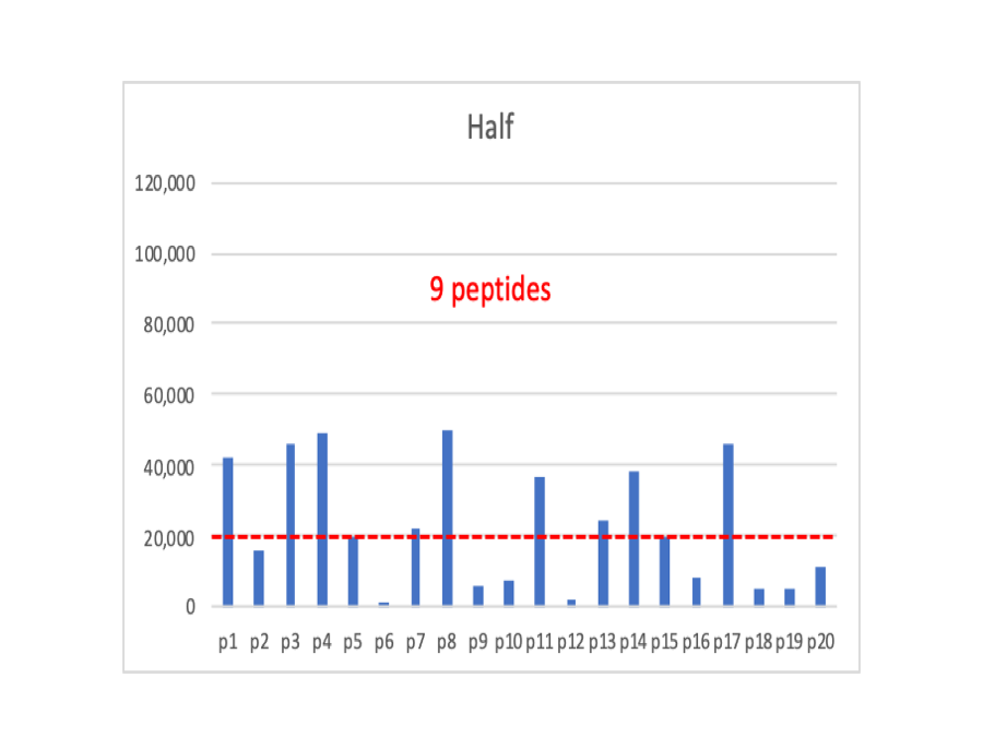
Now we have cut the overall intensity values in half, and we have 9 peptides above the dotted line.
If we cut the signals in half again, we now have just 5 peptides above the cutoff. Any more decrease in signals and we will no longer see the protein at all.
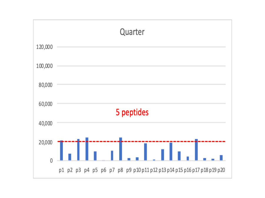
I made a claim above that shotgun quantification is just weighted spectral counting. So we will do the most simple thing that we can and just sum up the intensities for all of the peptides that are above the detection limit into protein total intensities. In the Full case, we sum up 13 intensities, in the Half case we sum up 9 intensities, and in the Quarter case we sum up 5 peptides.
Do we sum up all signals from all PSMs all of the time? No, we want to exclude any shared peptides. In what context are we defining shared and unique peptides you might ask? The answer is in whatever final protein context that we deemed appropriate for the results. Remember that the changing contexts involve tradeoffs. In many cases, if we sacrifice a little protein quantification resolution, we can dramatically increase the fraction of peptides that are unique (in that context). Check out Section 3.4 on Quantitative Information Content in Ravi’s thesis for more details and some examples.
Data quality, as measured by a few metrics, improves as we aggregate from the PSM to the peptide level and as we go from peptides to proteins. We explored those improvements in this dilution series notebook. That data is one mouse brain sample digested and labeled with 6-plex TMT and then combined in 25:20:15:10:5:2.5 relative volumes across the channels. There are 60K PSMs, 20K peptides, and 2,700 proteins. The protein total intensities span 7 orders of magnitude in intensity. It is kind of the product of the 2-3 orders of magnitude in spectral counts times the 4-5 orders of magnitude of individual PSM intensities.
Does this protein rollup work?
That is the 64 thousand dollar question. There are a lot of proteins in the world and biological systems seem to enjoy finding unusual ways to solve problems. There are no doubt hundred (maybe thousands) of journal articles detailing cases where all of this falls flat on its face. If you can think of your favorite example and pinpoint exactly where these protein rollup efforts fail, the we have made some real progress. Discovery quantification is not the answer to every question. Understanding its compromises and tradeoffs is crucial to knowing when not to use it. There are tradeoffs to targeted quantification, too, and it is not the solution to every problem either.
Can we try and answer if protein rollup works or not? These kinds of questions are truly one of the challenges in proteomics method development. We almost never have any systems with truly known outcomes. Common ways to try and address such questions are to make artificial test mixtures where the outcomes are known. These are usually spike-in mixtures that address quantification dynamic range and accuracy rather than overall sanity. These typically fall into the positive control category. The most common drawbacks are that the mixtures can be too simple to mimic the real biological samples, and many times the spike-in proteins are medium to higher abundant proteins. Most of the warts in proteomics methods are from the lowest abundance proteins where the information gets too sparse to test anything.
If you have done any normalization methods work, you learn to ignore the proteins that are changing in abundance. They are just a nuisance. The meat and potatoes are the proteins that are not changing in abundance. They are the critical proteins that nearly all normalization methods absolutely have to have to work. The sources of variation that we are trying to remove in the normalization methods cause the measurement of a constant (the expression level of an unchanging protein) to be variable between samples. We adjust the data in ways designed to make those constant values converge. These unchanging proteins are a negative control that we can exploit in the actual experiments we are most interested in studying. We can do sanity checks on real data without having to rely on test mixture data that may be a poor proxy for real cases.
Some sanity checks from TMT data
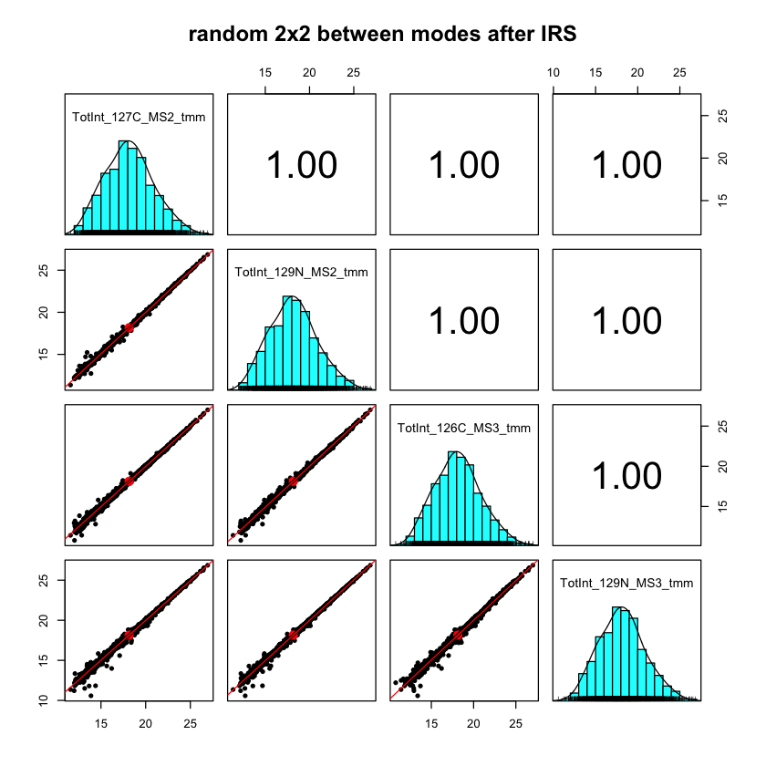
This paper by D’Angelo et. al added 13 spike-in proteins to an E. coli digest background. Ten TMT channels were used and the data was acquired using the SPS MS3 method and a more conventional MS2 method. The notebook looks at the data characteristics for each acquisition mode and even uses IRS normalization to directly compare SPS MS3 data and MS2 data. We are measuring the same E. coli digest in each channel (the spike-in proteins were ignored). In the figure below, we are making scatter plots of 4 randomly selected channels out of the 20 (2 MS2 reporter ion channels and two SPS MS3 reporter ion channels). We see nearly identical rolled up protein intensities over a wide dynamic range with some small deviations for proteins at lower abundance (where the numbers of PSMs contributing to the protein totals becomes smaller).
Internal reference scaling (IRS) is a method I developed to put multiple TMT plexes onto a common intensity scale (described here). The data for this notebook is from a 60-sample study that needed seven 11-plex experiments to accommodate all of the samples and internal standards. We had three extra channels (one each in three of the plexes) where we labeled an extra replicate of the pooled internal standard. We can use these three channels as canaries in a coal mine to spy on the IRS procedure.
The abundance estimates for each protein in the pooled standard (over the full range of detection) are the sums of the unique peptide reporter ion intensities. Those estimates have to be accurate to correct for the random MS2 sampling and make the measurements of the pooled standards the same in each TMT plex. Since we are using two channels of each TMT for the pooled standards for the IRS corrections, we cannot use them for any quality control. They end up very similar after IRS mostly because of the mathematics (see this notebook for more on that point). However, we can use the three extra channels (that were independent of the channels used for the IRS method) to see if we can successfully measure the same thing and get the same value.
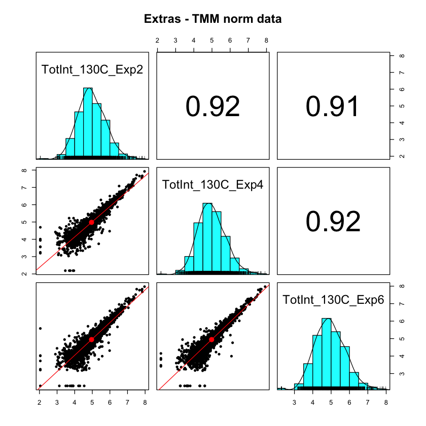
These are the rolled-up protein intensities of the three extra standard channels after the best conventional normalization methods. These are supposed to be identical samples but the sample-to-sample scatter plots are terrible. This distortion is because MS2 scans are not always at the same relative elution time (like the apex). The IRS method corrects for that specifically.
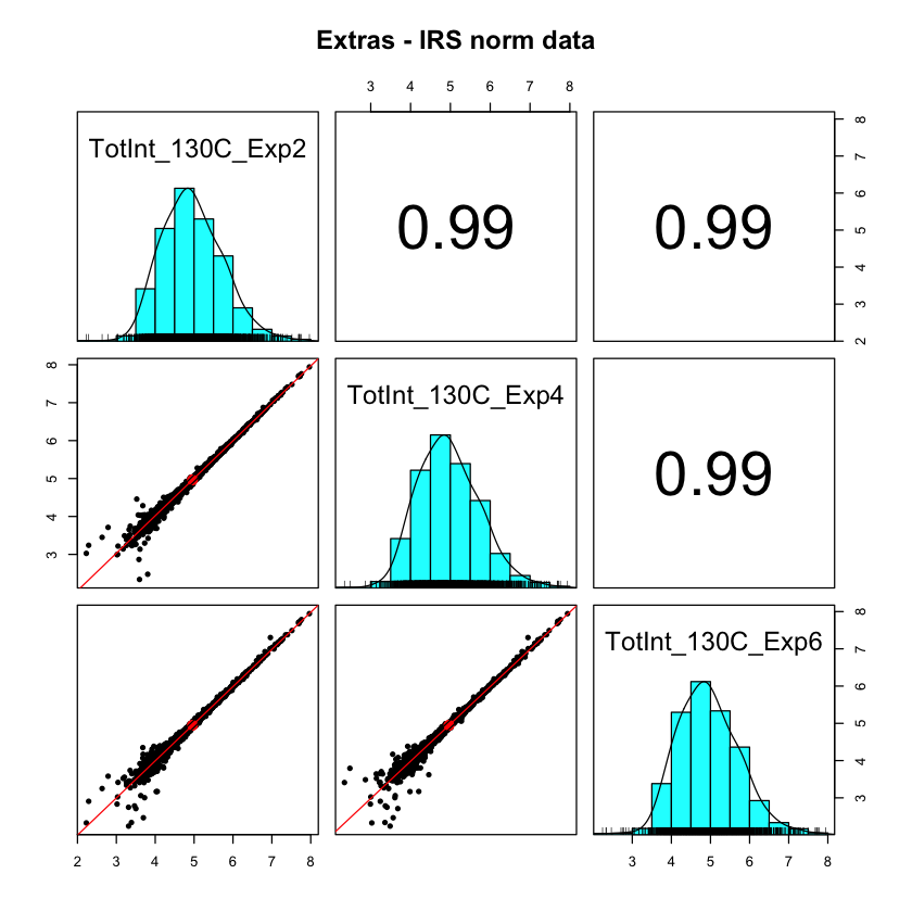
After IRS (which did not use these three channels), we now have very consistent protein totals over the upper 4 decades of intensity. It is only in the lowest decade that we start to see some deviations from identical. The samples were urine exosomes from human subjects and there was a great deal of biological variability.
Each TMT plex was a 30-fraction experiment. The numbers of PSMs associated with each protein will be different in each experiment. We are not imposing any requirements that we see the same peptide sequences for each protein. The sets of PSMs could be different between experiments and it would not matter as long as we still had a protein total intensity. This is why I said that “sum everything up” methods are more forgiving.
When are these assumptions violated?
Shotgun quantification studies are often trying to compare protein abundance measures between samples. Shotgun techniques (by definition) are looking at pieces of proteins. We can only see the types of protein pieces that are in the theoretical search space (that is how search engines work). Search space is defined by the protein sequences in the FASTA file and by the search engine parameters.
The FASTA file might be a canonical set of gene products (one representative protein for each gene). That would probably exclude any potential isoform information. Even if isoforms are present in the FASTA file, low sequence coverage for most proteins would not result in isoform distinguishing peptides to be seen for the majority of the proteins. Isoforms for most proteins will be invisible after digestion because the chance of detecting distinguishing peptides is too low.
Including non-enzymatic cleavage sites and/or large numbers of post-translational modifications dramatically increases the number of peptides in the theoretical search space. This can make searches too slow to be practical and can increase the chances for false positive results. These two factors are independent so their negative effects are multiplicative. For PTM searches, there can be be instrumental requirements (fragmentation modes, accurate fragment ion masses, etc.) that might be at odds with the quantification method. We need very specific instrument requirements to do SPS MS3 TMT, for example.
We need to start with some sort of a lowest common denominator situation and see where to go from there. That might be using a canonical FASTA file, full or semi-tryptic cleavage, static modifications for any labels, and unmodified peptides with variable oxidized methionine. These parameters should catch most of the protein pieces so that the rolled up protein values will be good estimates of the protein abundance for the vast majority of the proteins in these discovery experiments.
There are always exceptions to rules. We could have a protein become extensively modified in disease, such as Tau protein in Alzheimer’s disease. We might see a decrease in total protein signal because we have lost unmodified peptide signal to new m/z values (the modified forms) that we cannot identify because of the search engine parameters. The decrease in unmodified peptide abundance can be used to estimate the total amount of modified forms (FLEXITau method). If we had unchanged expression of Tau protein between conditions, but had an increase in modified peptide forms, we would observe a decrease in protein signal. That could be mis-interpreted as decreased protein expression instead on an increase in PTMs.
We can also have protein processing (truncations) associated with disease. We might have an actual difference in the protein sequence present in the samples from different conditions. A shorter protein form would likely have fewer peptides and a rolled up protein signal could be smaller that from a longer protein (assuming equal expression levels). We might again see a pattern that looks like a decrease in protein expression that is really an increase in truncation.
We could probably think of situations like these until the cows come home. We need to better understand and communicate potential limitations to clients and collaborators. In a core facility, it is impossible to have the detailed domain knowledge for every system to explore all of the possible limitations. The clients, who are the experts on their systems, are the ones who need to think about these issues. They need some working knowledge of the shotgun quantification process and its assumptions to decide if it is appropriate for the questions they want answered.
Questions about isoforms, variants, PTMs, etc. are really things to be explored after we have learned something from simpler differential protein expression studies. They need to be addressed in separate follow up experiments and analyses. A quantitative shotgun experiment is not always the best thing to do (and certainly not the only thing to do). That is why there are other methods like top-down and targeted analyses. If you already know what you are looking for, then the shotgun fishing trip is probably a waste of your vacation time (i.e. not the best use of sample, instrument time, or analysis time).
Thanks for reading. Phil Wilmarth, September 21, 2019.